The Problem with Gerrymandering
Gerrymandering doesn't just produce ugly maps. It reduces the number of genuinely contested elections, pushing representatives toward the extremes and away from the voters in the middle. The diagram below shows how different redistricting strategies affect the number of competitive districts — and therefore the health of democracy itself.
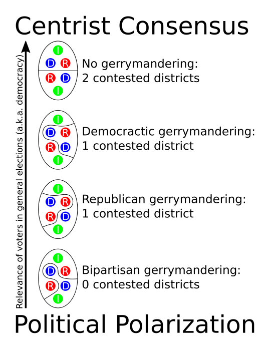
How different redistricting strategies affect contested elections. Gerrymandering — whether partisan or bipartisan — reduces competition and accelerates polarization.
The Convex Optimal Solution
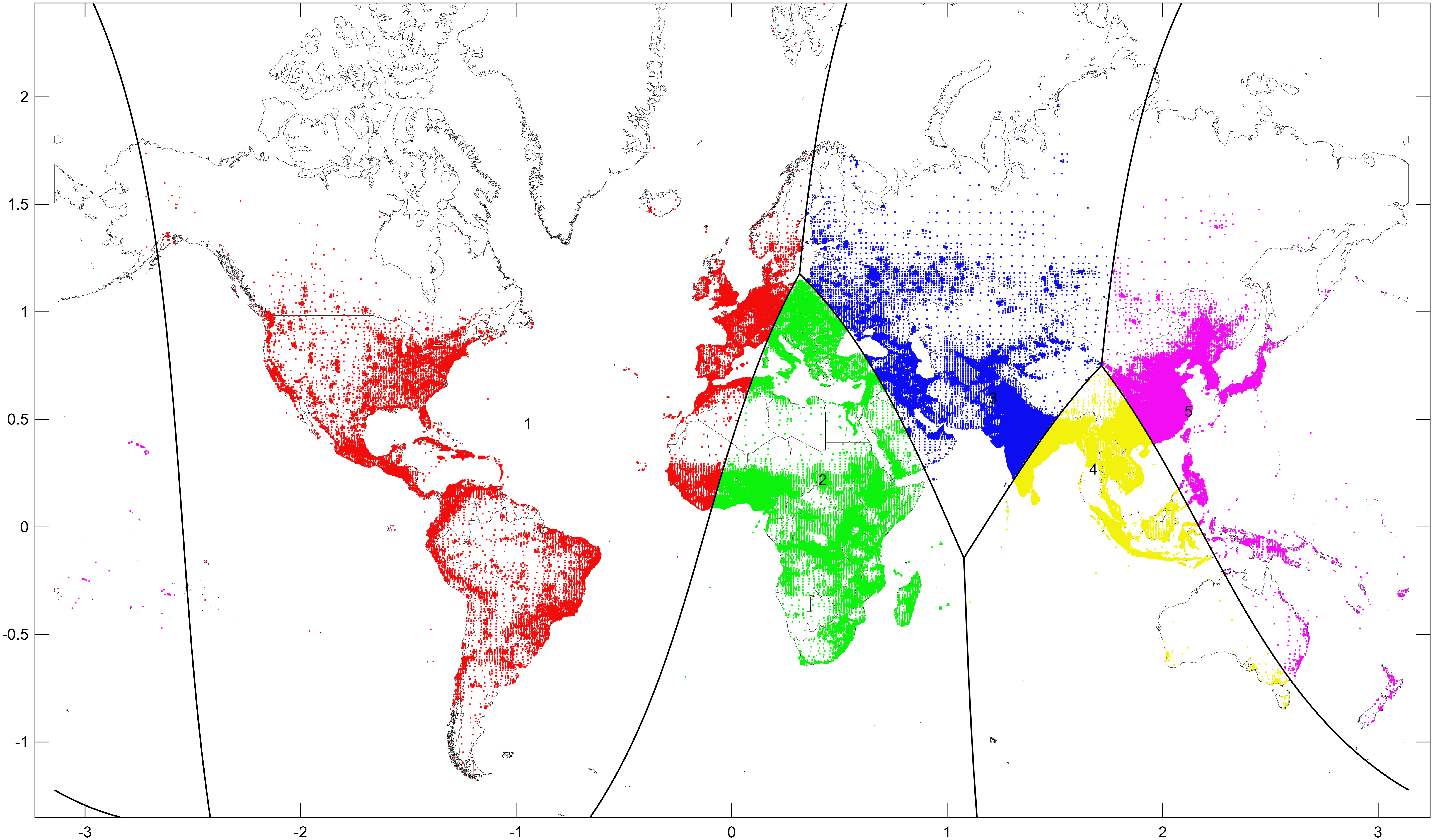
The key insight is simple: if the algorithm doesn't know how people vote, it cannot gerrymander. Convex optimal districting takes only population geography as its input — where people live, nothing else. It then finds the unique partition of the state into districts that minimizes the average distance from each person to their district's center, using a notion of "average" that guarantees every district is convex.
Because the solution is mathematically unique, there is no room for manipulation. The map draws itself.
The Algorithm
The method works iteratively, refining districts until they are both equal in population and geometrically stable:
Start with random initial district centers placed across the region.
Assign each population block to the center minimizing f(distance to center) − bias, where f(x) = x² for flat geometry and f(x) = ln(sec²x) for spherical geometry. The bias controls population balance.
Measure population imbalance. Increase the bias for underpopulated districts (making them more attractive, so they grow) and decrease it for overpopulated ones (making them less attractive, so they shrink). Keep doing this until equal populations are achieved in each district.
Move each center to the population-weighted point that minimizes the average f(distance) to all assigned population blocks.
Repeat steps 2–4 until districts are equal in population and boundaries stop changing.
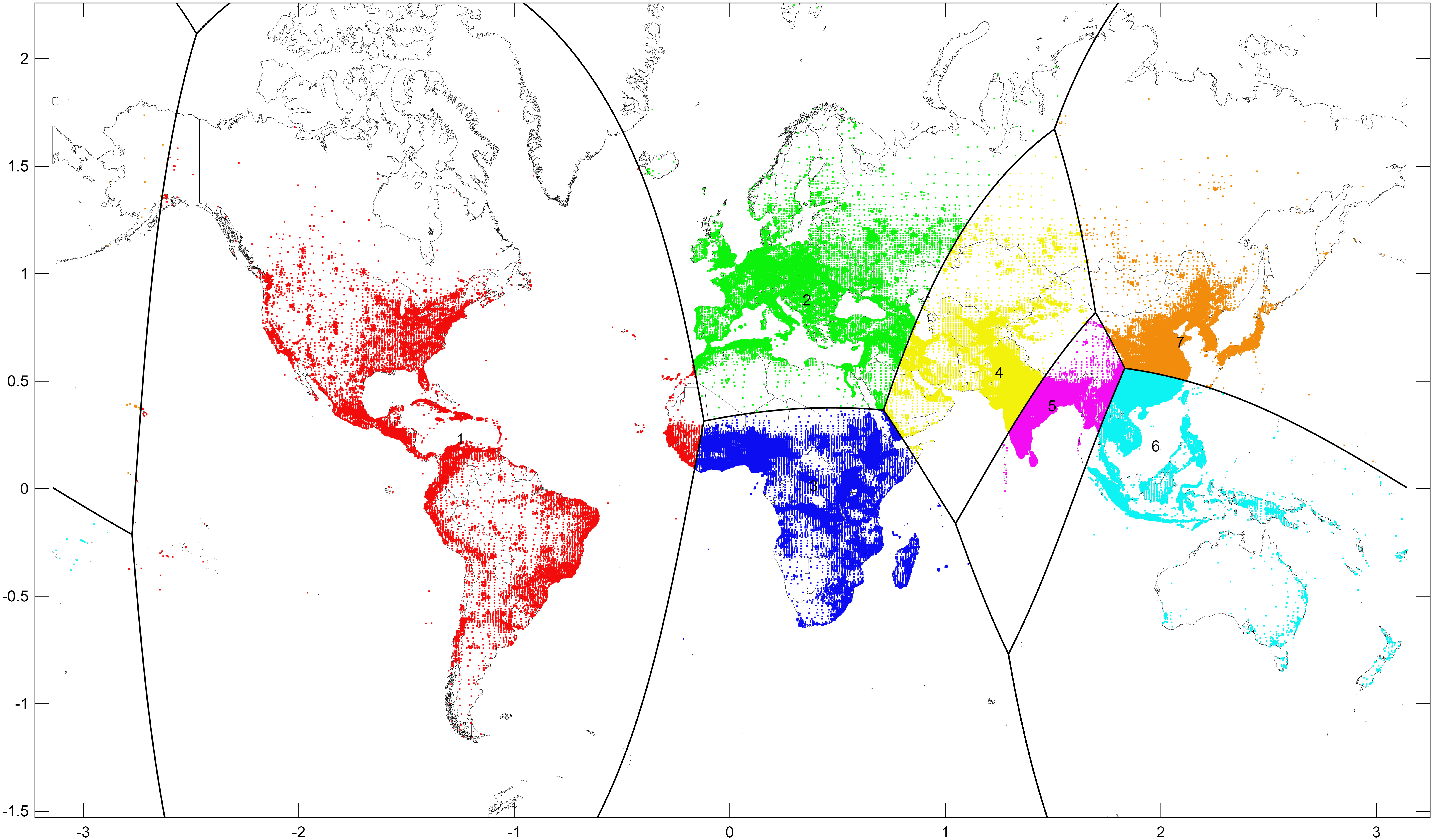
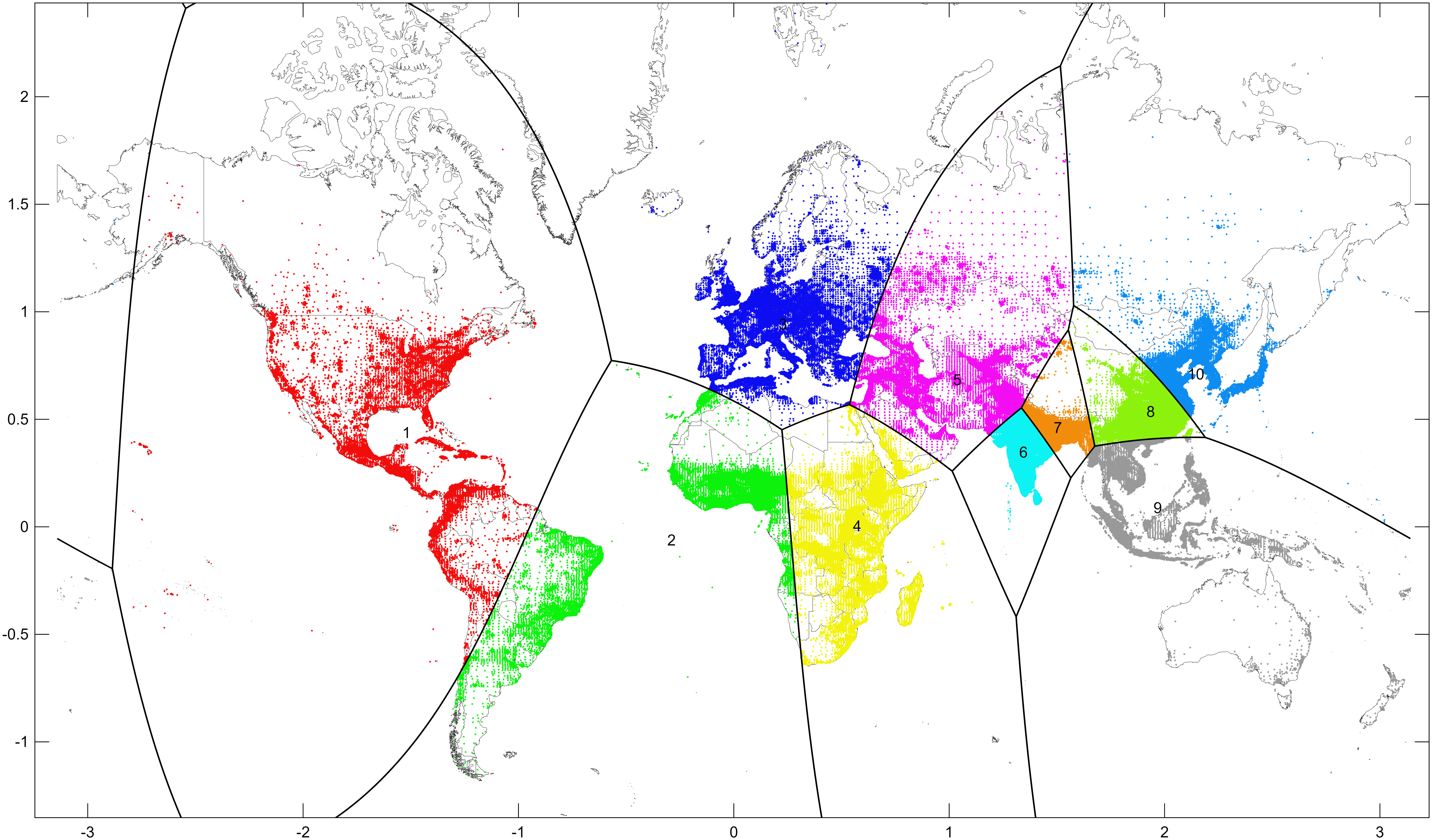
The result is a set of districts that are compact, convex, and equal in population — determined entirely by where people live.
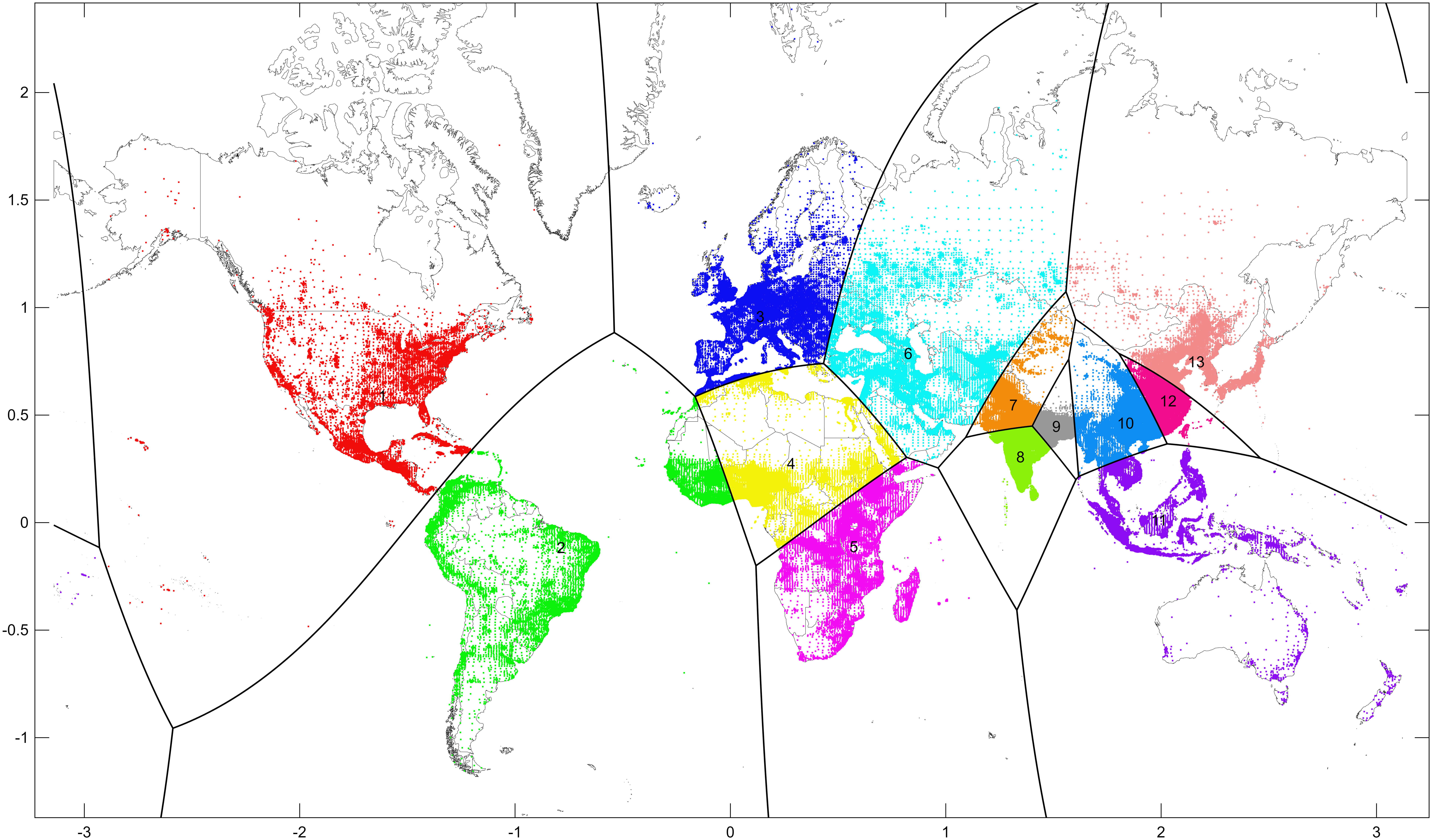
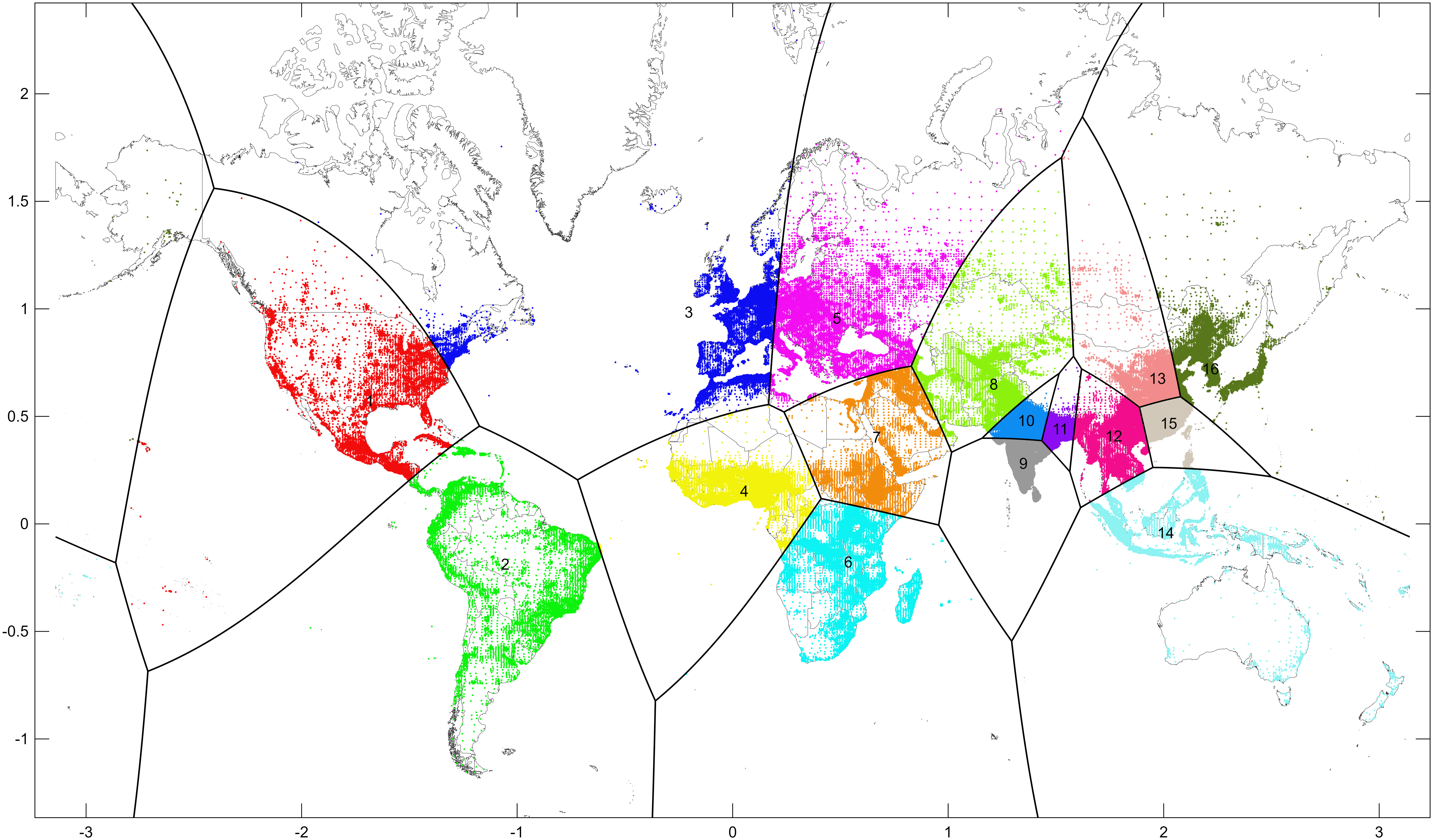
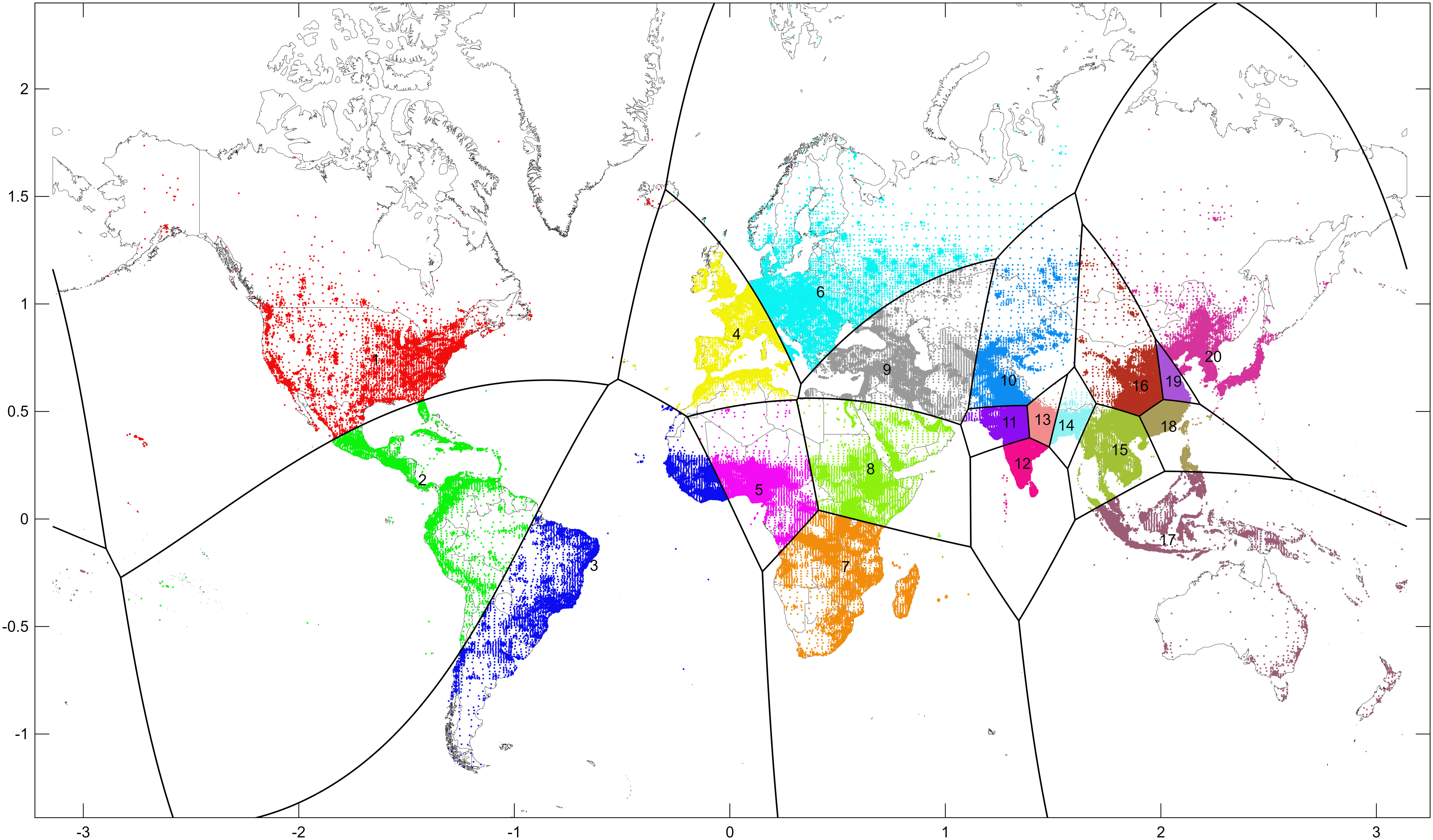
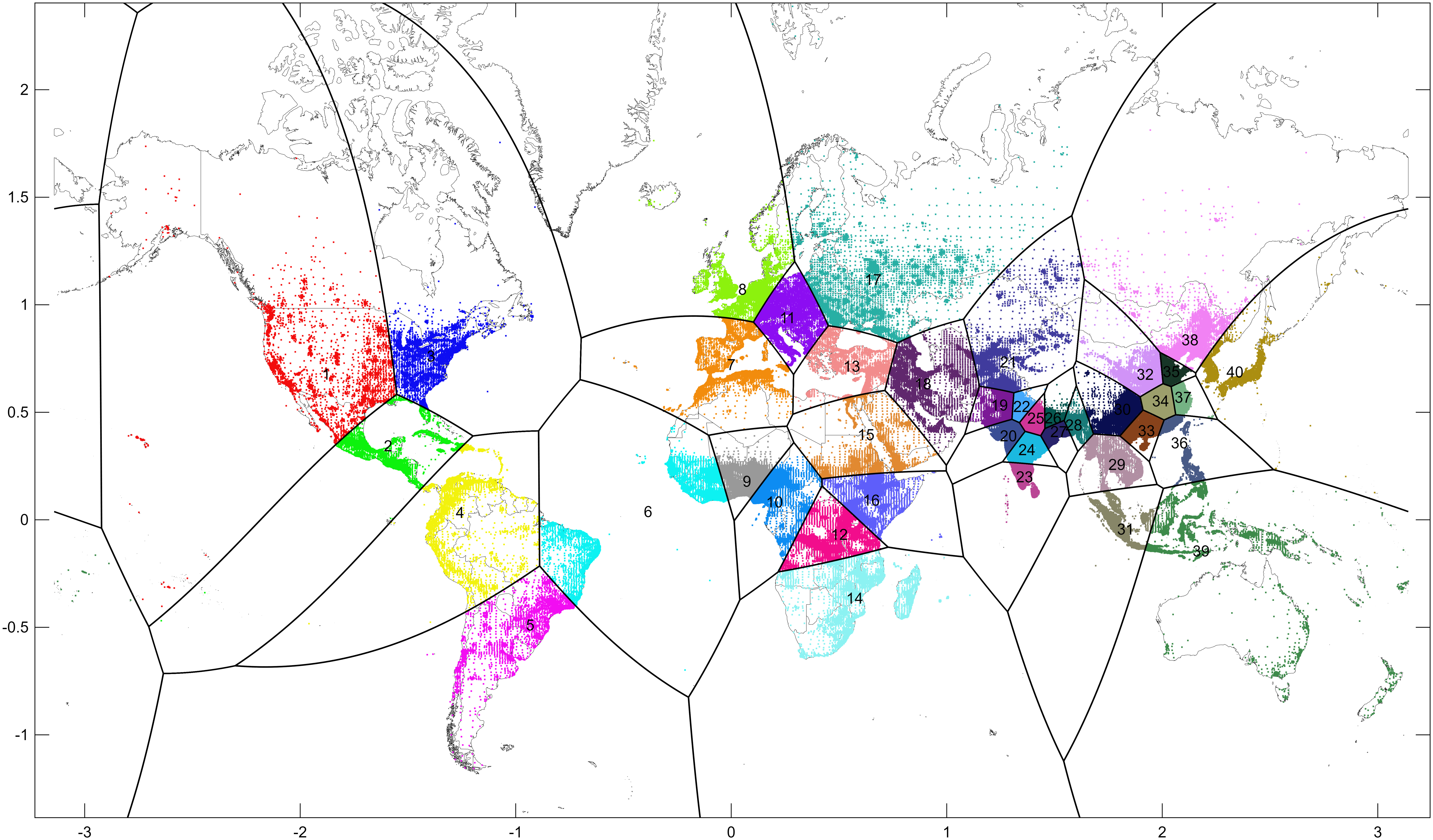
The Earth, Partitioned
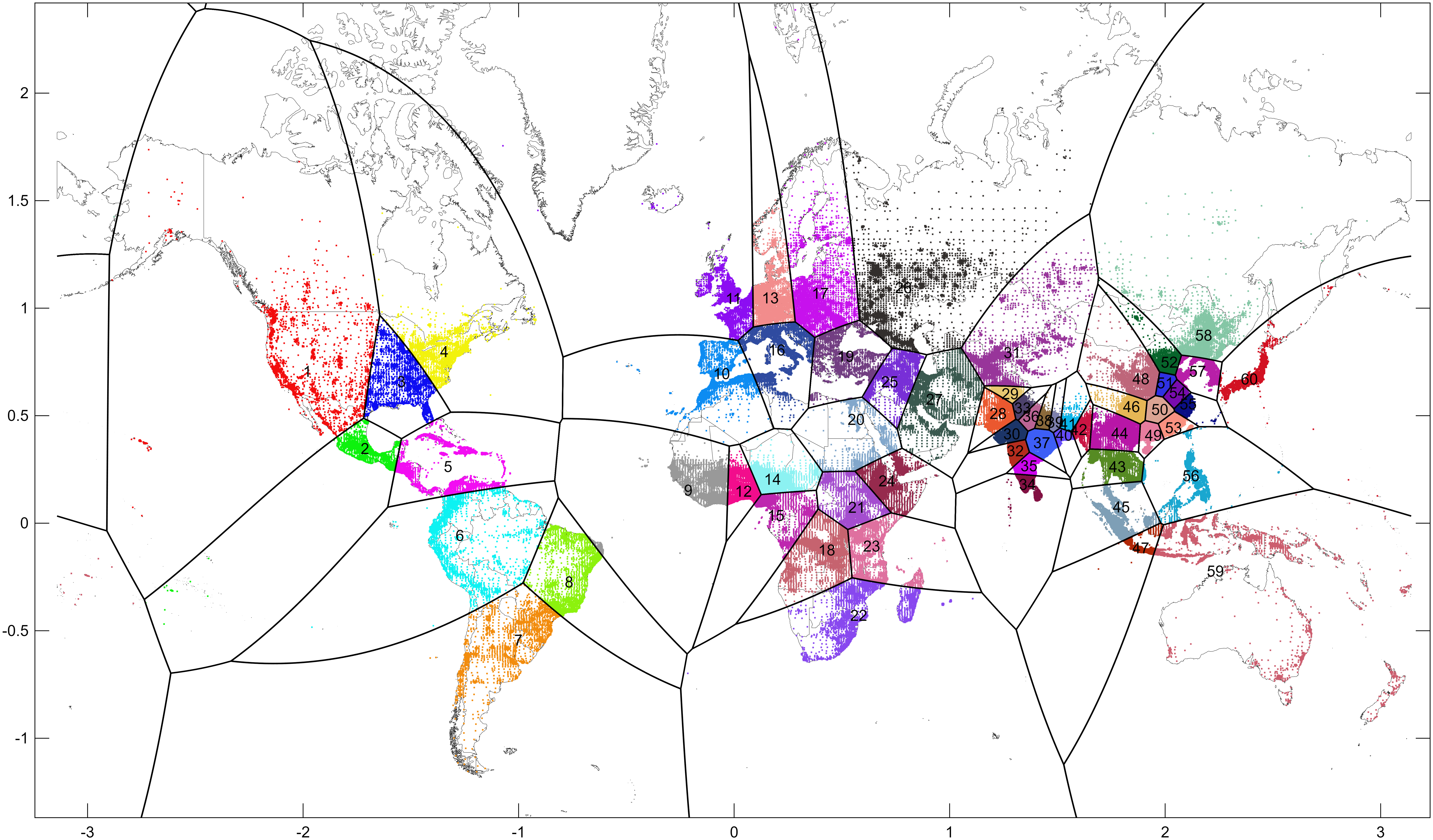
For the Mathematically Curious
The following section presents the mathematical foundations of convex optimal districting — why squared distance produces straight boundaries on a flat map, and why a modified distance function produces great-circle boundaries on a sphere.
Why the Boundaries Are Straight
The diagram below shows the key insight: the same algebraic structure that makes d² produce straight-line boundaries on a flat surface has a spherical counterpart — using ln(sec²d) — that produces geodesic (great-circle) boundaries on a sphere. This means the algorithm works correctly on the curved Earth, not just on flat maps.
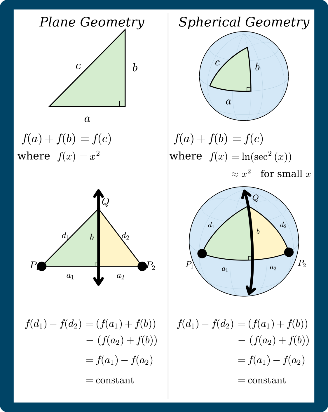
Left: flat geometry where f(x) = x². Right: spherical geometry where f(x) = ln(sec²x). In both cases the same algebraic cancellation produces straight boundaries.
The Energy Function and Equal Population
Shows why the bias terms enforce equal population — and then vanish entirely from the solution.
The algorithm minimizes (over centers and assignments) and maximizes (over biases) the following energy function. For concreteness, consider 8 regions and 24 population points:
where Xi is the i-th population point, Ck is the center of region k, bk is the bias for region k, and κ(i) is the assignment of point i to a region. The function f is f(x) = x² for flat geometry and f(x) = ln(sec²x) for spherical geometry.
Taking the partial derivative of E with respect to bk and setting it to zero:
This forces each region to contain exactly 3 points — equal population. The equal population constraint is not imposed externally; it emerges naturally from maximizing E over the biases.
What is an average distance with respect to f? Consider a simple example: what is the average of 1 and 7? The usual answer is (1 + 7)/2 = 4. But with respect to f(x) = x², it is \(\sqrt{\frac{1^2 + 7^2}{2}} = \sqrt{\frac{50}{2}} = \sqrt{25} = 5\). This f-average gives extra weight to larger values because squaring amplifies them.
Why use this unusual average? As shown in the proofs above and below, only by minimizing the average distance with respect to f(x) = x² on a flat surface — or f(x) = ln(sec²x) on a sphere — do the boundary equations reduce to straight lines. Convexity is not an added constraint. It is a mathematical consequence of the choice of f.
The min-max argument guarantees a local minimum, not necessarily a global one. Different starting configurations may converge to different solutions. To find the best map, the algorithm is run many times from random initial district centers, and the solution with the smallest value of E — the smallest total f(distance) — is selected. This is the convex optimal solution.
Proof: Straight-Line Boundaries on a Flat Surface
Minimizing squared Euclidean distance produces linear boundaries between any two regions.
Let C₁ = (x₁, y₁) and C₂ = (x₂, y₂) be two centers with biases b₁ and b₂. The boundary is the set of points where both centers are equally attractive:
Expand using the standard Euclidean formula:
Only linear terms survive, matching the standard form Ax + By + C = 0:
The biases shift the line's position but introduce no curvature.
Proof: Geodesic Boundaries on a Curved Surface
Replacing d² with ln(sec²d) recovers straight boundaries — great circles — on a sphere.
Let C₁ and C₂ be two centers on the equator with biases b₁ and b₂. The boundary satisfies:
On a sphere, d² = p² + h² becomes the Spherical Pythagorean Theorem for a right triangle:
Apply the secant identity and take the natural log. Multiplication becomes addition:
This is the Curved Pythagorean Theorem in additive form — structurally identical to the flat case.
Where h is the shared off-axis height above the equator:
In this setup, with both centers on the equator, the boundary depends only on p (position along the equator), not on h (height above it). Since the solution is independent of h, the boundary does not curve as you move away from the equator — it forms a meridian, perpendicular to the equator and to the line connecting the two centers. A meridian is a great circle.
In the general case, where the two centers are anywhere on the sphere, the same algebraic cancellation occurs along whatever great circle connects them. The boundary is always a great circle arc — the straightest possible line on a curved surface — perpendicular to the great circle connecting the two centers.
References
Cohen-Addad, V., Klein, P. N., & Young, N. E. (2018). Balanced power diagrams for redistricting. arXiv preprint arXiv:1710.03358v3.
NASA GPW v4 (2020) Population Density Data. Global grid of population estimates.
U.S. Census Bureau (2020). Redistricting Data (PL 94-171). Official block-level population data.
Convex optimal maps and proofs by Andrew Bray. World partition maps computed in MATLAB.